If you are like me and usually updates manually a spreadsheet to track your progress in a daily basis related to something like diet or spenditures, you will know that your spreadsheet may become very long. That’s why I created an small script to allow me jump to current date cell on Open in Google Sheets automatically.
The script will run like a macro and after a few moments you have opened the spreadsheet, it will focus the correct cell!
Preparing your file in Google Sheets
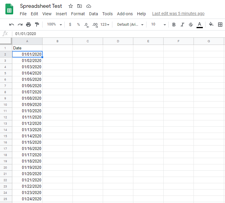
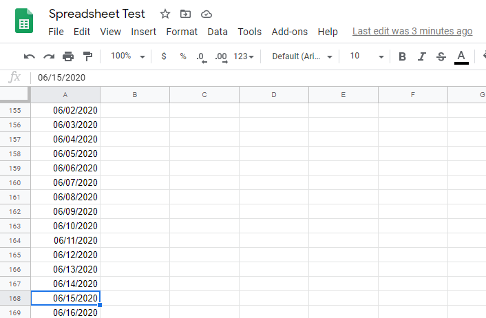
You need to setup a file first and prepare the data. Here you can see in my example that in the range “A2:AN” we got the dates for each one of the days of 2020.
Creating the script to perform cell focus on Today date
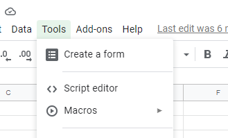
Once you got the file working, you can go ahead and click in Tools -> Script editor.
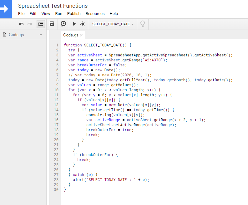
A new tab will be opened. In this new tab you can paste the script below, then give a name for your project and hit Save!
The script just need to be changed by you on the line 4. There you should replace by the correct range that you want to search.
Adding the trigger jump to cell on Open
Once saved you can now proceed to configure the project triggers, so the function will execute properly. In order to access these configurations, you need to click on Current project’s triggers.

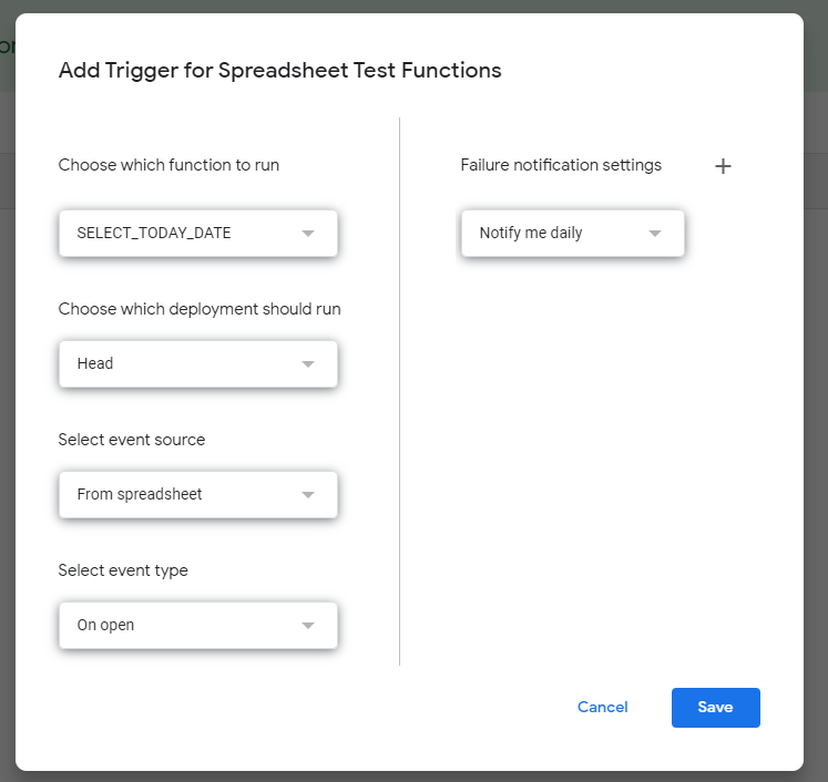
On the new tab that will show up, you must click on Create trigger and configure it based on your data following the example below:
After that you can go ahead and just confirm the screens that will be presented. If by any chance you see this screen, just click on Show Advanced and then in Go to “project name” (unsafe). You can learn more on verifying your scripts accessing Google documentation.

Once
That’s it! I hope this blog post can help you on setting the function to jump to current date cell on Open in Google Sheets.


Hi, thanks for this tutorial!
Works a treat and makes reading our shift rota much easier. Just a quick question, is there anyway the resulting day is shown at the top of the window instead of at the bottom?
Thanks
Steve
Hey Steve! Good to know that it helped you. I have a spreadsheet to track working hours and it was boring to select the current date every day. So I decided to come up with this script.
I like your idea and I decided to update the script with this new behavior. You can try the new script in this same post.
Thanks!
Wiliam
Worked like a charm! Thanks
Glad to help you sir!
Hi William,
I can’t get this to work. My dates are listed automatically in UK fashion (day, month (name, not numerically), then year).
Can you help?
Many thanks,
Charlie
Hey Charlie!
In order to make the changes for you to support this type of format, could you confirm if the date looks like ’04 JUL 2021′, ’04/JUL/2021′ or ’04/JULY/2021′?
Thanks!
Hey William,
Thanks, this was exactly what I needed! However, I cannot get it to work. My date format is “7/12/2021” and formatted as a date type. I changed the range and added the trigger as instructed… (BTW also had to “Import” the script on Tools -> Macros -> Import).
Any help?
Thanks
Matt
Hi William,
It worked for me which is wonderful!
However, it works only the first time I open the sheet and visit a tab. But it doesn’t execute when I click on subsequent tabs which also have dates in column A. Is there a way to make this execute on a per tab level instead of executing once the first time I open the sheet? I could refresh the screen after I move to another tab but then I wouldn’t really be saving much time if I just instead scroll down to Today’s date.
This is exactly what I’m looking for but can’t get it to work, when I run it it’s executing fine but nothings happening on the actual sheet, I’ve made sure my dates are formatted as such and all the fixes I see people receiving in the comments, where might I look to figure out what needs doing?
Hey,
This works awesome!! I have frozen rows and columns how do I make sure the first row stays visible?
Thanks,
Hey,
If you are mentioning the first row as header, I believe it will remain visible always. But if it is the first row with data, then I think you should freeze two rows then, the header and the first row hahaha
Best,
Wiliam
Hi Wiliam Rocha,
Works as expected, thanks a ton!
Keep up the good work.
Good Luck!
Thanks for the feedback, Pankaj! Glad it worked for you 🙂
This is well done… what I would like to see is a version where it opens to the next date > today… basically the first date value it finds in column A that is greater than today’s date.. ie, the next valid date in the future in Column A.
Hello Django,
Thanks for reaching out.
The version should be any next date or just the next day?
Best,
Wiliam
Thank you for creating and sharing this script. This was my first scripting experience and your instructions were clear and helpful. Oddly it worked the first time then I had to disable Adblocker the second run and fine since.
It works as described when the file is opened in Google Sheets.
The sheet I am scripting is shared with preview setting and embedded in a course LMS. The script does not activate when a button is clicked to display the schedule.
What do you suggest I do?
Hey Daniel,
I never tested like that before, but I think we have some options. Basically, you want to trigger the current date cell selection when you press a button outside of embedded frame?
If so, we need to make some changes to listen for clicks that happen outside of the frame and then trigger the auto selection again, not only during the Spreadsheet Loading.
You can reach me via email so we can discuss more.
Best,
Wiliam
Hello William, what modifications to the script can we do if our dates run horizontally across the sheet? In my instance, I’ve changed the range to getRange(“B1:H6250”), however I am not knowledgeable in scripting by any means, I do not know if it is possible to modify your script for my use. Please advise, thanks!
Hello Joel,
Thanks for reaching out!
I have updated the script so it can work with your range as well 🙂
Best,
Wiliam
This script looks like it has potential for my use case, but instead of a date value in a cell, I have a function that supplies a dates for the month across a row, which is hidden (protects raw date calculation).
When someone opens the spreadsheet, I would like to have the column with date equal to or immediately following the current date (today) to display on the left.
Hello Shawn,
I believe the script as it is will work for your scenario if you define the hidden range of cells in the line:
var searchRange = activeSheet.getRange(“B219:F220”);
Also, you will need to a plus one in the step that activates the range:
activeSheet.getRange(x + 1, y).activate();
I think it can work for your use case.
Best,
Wiliam
Hello – I use the date formal day/month/year (e.g. 24/09/2022). How should I adjust the script. I don’t get any error messages, but it doesn’t seem to work. Thanks
Hi Colin,
Could you check if the cells are formated to use Date type? Or they are in General or Text type?
Best,
Wiliam
Got it to work!
I used this code:
“`
function openToDate() {
const sh = SpreadsheetApp.getActive();
const ss = sh.getActiveSheet();
const dateData = ss.getRange(“C2:C366”).getValues();
const today = (new Date()).setUTCHours(0,0,0,0);
let d;
for (let i = 0; i < dateData.length; i = i + 14){
for (let j = 0; j < dateData[0].length; j++){
d = (new Date(dateData[i][j])).setUTCHours(0,0,0,0);
if (d === today){
ss.setActiveRange(ss.getRange(i+30,j+3));
break;
}
}
}
}
“`
There is a typo in the code:
x = x = firstCellOfRange.getRowIndex();
should be:
x = x +firstCellOfRange.getRowIndex();
After I corrected that piece, it worked splendidly for me!
Thanks for the script and work on it!
Hi Sean!
Thanks for the feedback and the fix. I have updated the script as well.
Best,
Wiliam
Hi!
Complete newbie here. Done my best but not working. Used Apps Script in Google Sheets, copied the code in (adjusted the range to A4 : A9000), saved it. Added to my sheet using Extensions/Macros/Import Macro. It shows up and says it is running successfully – but nothing happens when I manually run it or when I open the file.
My dates are formatted DD/MM/YEAR
Help?
Hi Abigail,
Is your column using data type Date? Also, do you have frozen columns or rows?
Best,
Wiliam
Hello – I use the date formal day/month/year (e.g. 10/02/2023). How should I adjust the script. I don’t get any error messages, but it doesn’t seem to work.
Hi YY,
I believe the only thing you need to ensure is to format the column you are searchin as Date. Ensure the data type is Date and it should be handled automatically by the script.
I believe I have done everything correctly, but it’s not working. My date is formatted (as a date number type) Thursday , March 23, 2023. Any suggestions? Do I need to change the code at all since the DOTW is in my date as well?
p.s. I have never done this before and honestly have no idea what I’m doing lol.
Hi William. I followed your instructions and screenshots above. They don’t match the 2023 Layout of Google Sheets, but I got all the way to the end and the script does not work.
For Column A, I have a client’s name.
For Client B, I have their court date. This is who the whole sheet is organized chronologically
Columns C thru Z contain other information.
Do you have any suggestions on what I should do? Thank you!
Hello,
It works perfectely for newly opened window. Unfortunately we have multiple sheets with dates. How to make it working when switching between sheets?